Organizing

In this lesson, we’ll discuss how to organize both a project directory and an R script. While there’s no one exact way to do either, there are good practices that you should generally follow.

Organizing a project directory

We’ll begin with how to organize your course and project files.

A place for everything and everything in its place

Every data analysis project should have its own set of organized folders. Just like you might organize a kitchen so that ingredients, cookbooks, and prepared food all have a specific cabinet or shelf, so too should you organize your project. We’ll organize our course directory in a similar fashion.

But computers are pretty good at finding files, you say: you can use your machine’s search feature to look for what you need. If you don’t have that many files to look through, you might not be too bad at quickly scanning to find what you want either. If this is the case, then why bother organizing a project directory? Why not just dump everything — scripts, data, figures, tables, notes, etc — into a single folder (My downloads folder works just fine, thank you…)? If you need something, the computer can definitely find it.

So what’s the big deal?

The big deal is that you are thinking from your computer’s perspective when you should be thinking from the perspective of you, your collaborators (which includes your future self), and future replicators (which also includes yourself). Search features are nice, but there’s no substitute for being able to look through a project’s files just by looking through the project folders. When a project is well organized, it’s much easier to understand how everything — each input, process, and output — fits together.

A common directory structure

As a reminder, here’s basic directory structure for this class:

student_skinner/
|
|__ assignments/
|__ data/
|__ figures/
|__ final_project/
|__ lessons/
|__ scripts/
|__ working/

As you can see, we have a main directory (or folder — same thing) for the course called student_skinner. Your directory has a similar name, but with your last name: student_<last name>. That said, it could be named anything useful. This can live on your computer wherever you want to put it: on your Desktop, in your home directory, in another folder where you store materials for your other classes — wherever makes sense for you.

Inside the main course directory, there are subdirectories (or subfolders — again, same thing) for the different types of files you’ll collect or create this term. These subdirectories have self-explanatory names: PDFs for assignments go into assignments, PDFs for lessons into lessons and so on.

Note that this type of structure works well with research projects. Of course, you’re unlike to have assignments or lessons subfolders within a research project directory, but you almost certainly will have subfolders for your scripts, data, and figures as well as a working folder (which some people call scratch, like a scratch pad) where you can store odds and ends or practice new ideas.

You may ask: why these folders in particular or, why should I have separate data, scripts, and figures in my project directory?

Think about it this way. Following our kitchen analogy from before, we have:

• Ingredients (Inputs) - data
• Cookbooks (Processes) - scripts
• Prepared food (Outputs) - figures

Particular projects may require particular folders (for example, you may find it useful to have a special subfolder for tables or one for regression output called estimates). But in almost all cases, your project directory should have separate subfolders for your data, your analysis scripts, and any output you produce.

Great! How to I set this up?

You can create new directories using your operating system. For both MacOS and Windows, one of the easiest ways to make a new folder is to right-click on your Desktop and choose to create a new folder. You can then open this folder and continue right-click creating subfolders until you have what you need.

You can also use the RStudio Files tab (lower right facet) to create new folders. Even though we already have our course directory from GitHub, let’s practice creating a directory structure from scratch, so you can make your own in the future.

Let’s say I want to create a directory on my Desktop.

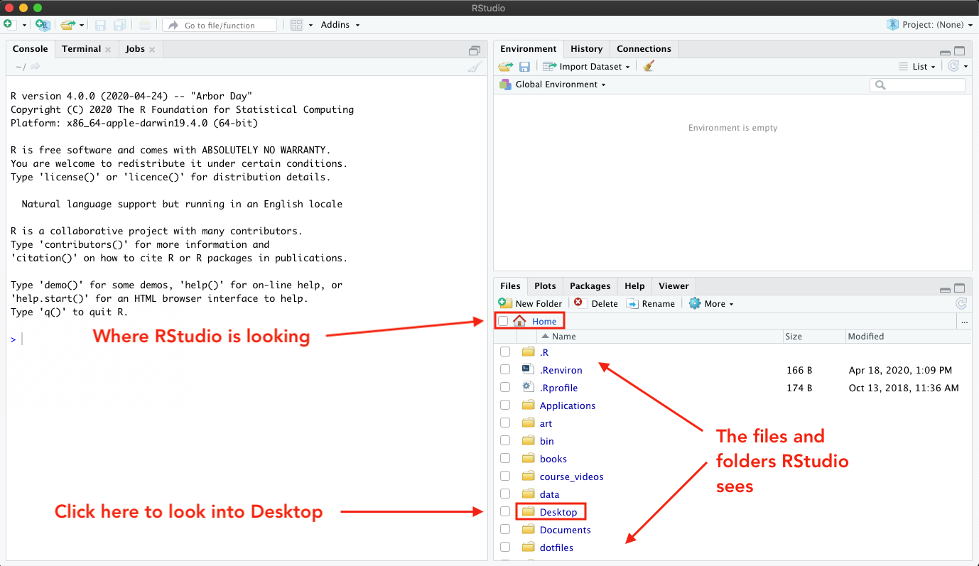
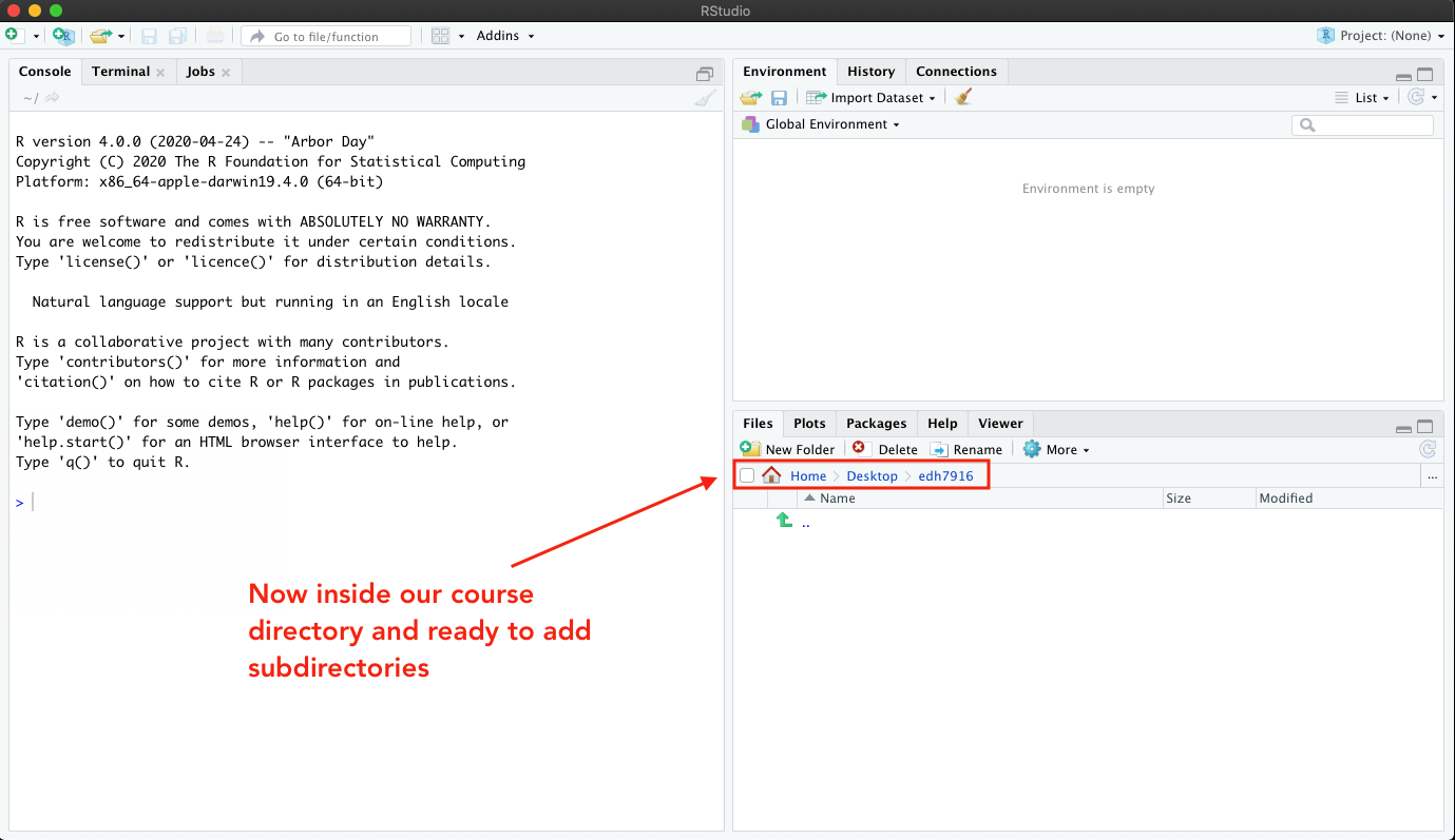
When I open RStudio, notice that it starts in my Home folder (we’ll talk more about what that means to “start in” below). You can see this by looking at the menu bar in the Files facet. It also helps that I can see all the folders and files listed in the window. Because I know generally what’s in my home directory (Applications, Desktop, Documents), it’s clear to me that that’s where I am. Depending on your settings, RStudio may start somewhere else for you — that’s fine, just check the menu bar.

So I’m in my home folder, but I want to be in my Desktop folder. Easy enough: I can just click the Desktop link in the window.

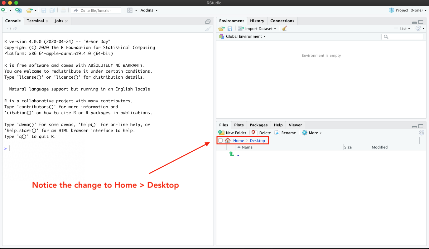
Notice how the file list has changed. There’s nothing there! That’s because I have a very clean Desktop! But if you have files on your Desktop, you should see those now. Either way, I can see that the menu bar address has changed to add a folder: Home > Desktop.

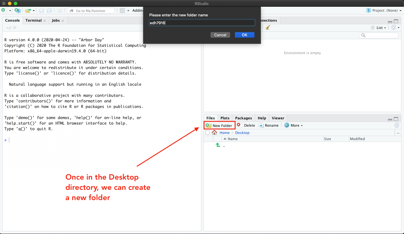
To create a new folder, I can click on the New Folder button and then give my new folder a name in the drop down menu. Let’s call it edh7916 to keep it separate from our student_* course directory.

Now you can see my new folder, which I’ve called edh7916.

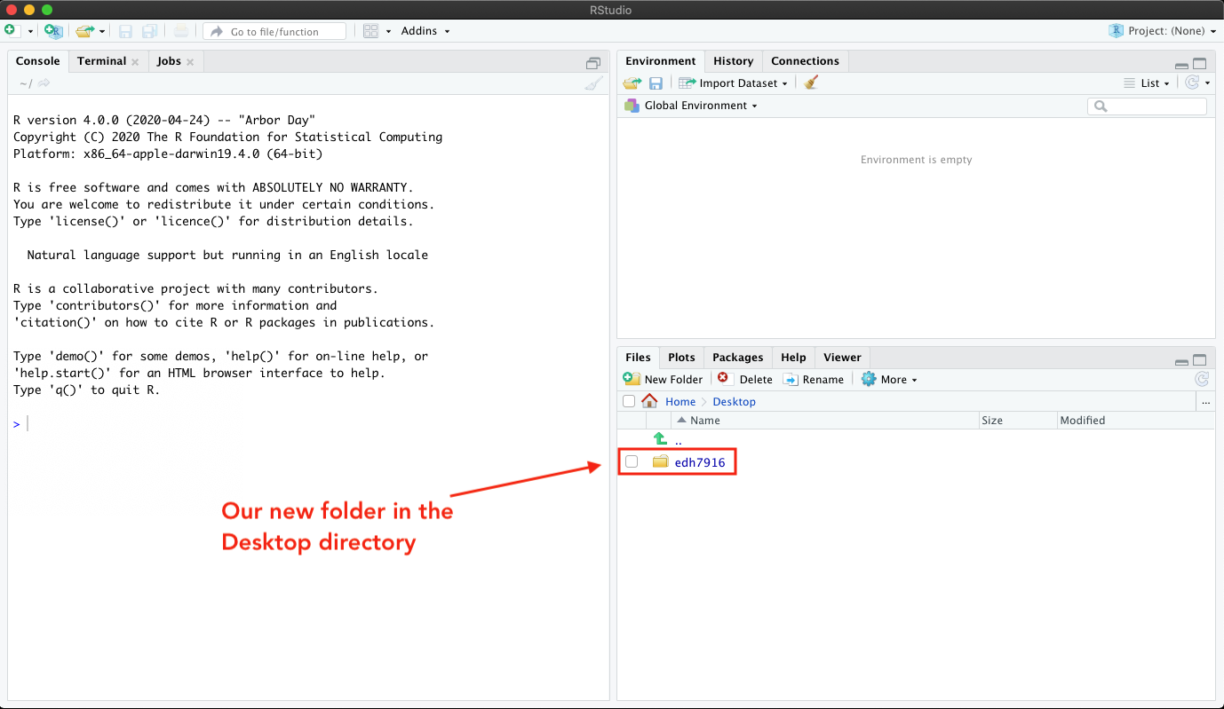
Clicking on that, I see the menu address change to Home > Desktop > edh7916 and nothing inside, which is expected since it’s a newly created folder.

Time to add the subdirectories!

Quick exercise

Fill out this directory with the following subdirectories:

• data
• figures
• scripts
• tables
• working

Quick aside into how applications find files

Above, I said

When I open RStudio, notice that it starts in my Home folder…

What does that mean, starts in?

There are two common ways to open a file on your computer with the correct application:

1. Open the application you know you need — let’s say Excel — and then choose to “Open…” an existing file from the main menu. When you go this route, a little window will open or you’ll see a drop down menu and will have to navigate to find your file.
2. Find the file you want open and then double-click it. On most computers, the correct application will automagically open and your file will be loaded (e.g. double click on an *.xlsx file and Excel will open with your file ready to go).

In this way, RStudio is an application just like any other application on your computer. If you double-click on *.R scripts or *.md or *.Rmd files, it’s likely that RStudio will open. However, if you open RStudio first, it begins by assuming you want to look for/store files in a default location — most likely your Home directory unless you’ve changed the settings.

This what I mean by starts in.

As you might be guessing by this point, how people set up their computers or organize their files will affect where RStudio needs to look for the correct files. One skill you’ll have to develop is being able to navigate to the proper working directory, that is, telling RStudio where your files are located.

Setting your working directory

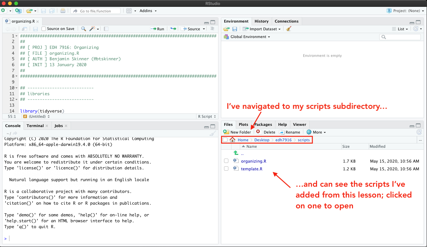
After downloading today’s scripts (the icons at the top of the page) and adding them to the scripts subdirectory of my course directory, I’ve opened one in RStudio (NB: You should already have these in your course repo from GitHub). Notice that we’re back to our student_* directory and not in the edh7916 test directory we made above.

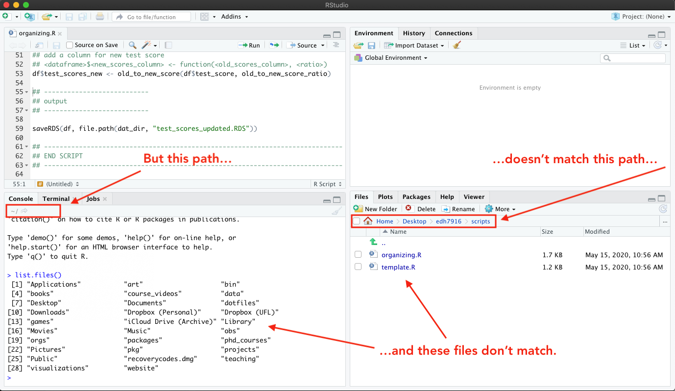
Despite what I see in the Files facet, however, my working directory is still set to my home directory. This means that when RStudio starts looking for files, it’s going to start in the home folder.

How do I know that? Notice that the path shown on the Console facet doesn’t match the one on the Files facet. Also, when I run the R function list.files() — which by default lists all the files in the current directory — in the console, I see the files in my home (~) directory rather than those I see in ~/Desktop/student_skinner/scripts directory.

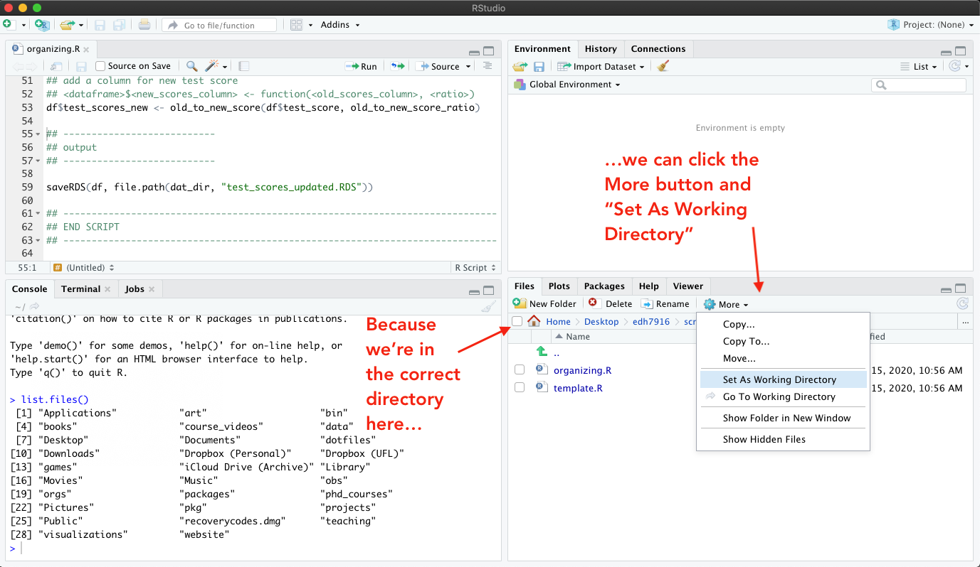
There are a number of ways to fix this, but the easiest way is to click the More button (with the gear) in the Files facet. In the drop down menu, you’ll see an option to “Set As Working Directory.” Because you are in the scripts directory, you can click it to correctly tell RStudio that you are working in scripts, not elsewhere.

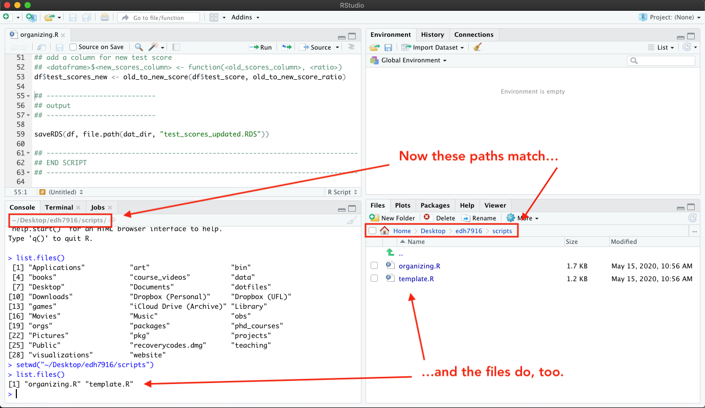
Clicking “Set As Working Directory” sends the command setwd() to the Console with the correct path to get from where RStudio starts to where you want to be. Now you can see that the paths in each facet’s menu bar match and when we run list.files() again, we now see the two R scripts listed on the left that we see listed on the right.

Now that you’ve found your course script files in RStudio, the next step is to understand how to make sure they can find your data and output folders.

Absolute vs relative paths

Every quantitative data analysis will need to coordinate the three ingredients discussed above (data, scripts, output). When your script attempts to read in data, it has be able to find it on your computer. Similarly, when it’s time to make a figure, its needs to know where to save it. In other words, you need to give it paths to your other folders.

There are two basic types of paths — relative and absolute — and which type you choose to use will affect the transferability and replicability of your work.

A quick analogy. Imagine you ask a friend for directions: how do I get to the state park? Your friend has three ways they can give you directions:

1. Directions to the park from their house
2. Directions to the park from your house
3. Directions to the park from a common landmark

The first way is really easy for your friend, but it puts extra work on you. Either you have to go to their house first so that the directions make sense, or you have to translate them from your perspective. Directions like these are annoying at best and useless if you don’t know how to get to their house.

The second way is really nice to you, but difficult for your friend. However, the directions aren’t as useful if you don’t plan to start from your house. In addition, these directions also aren’t reusable for other people — if a third friend tries to get the directions from you, you’ll just replicate the first problem for them.

The third way is the best compromise. If you each know how to get to a common landmark, then you can head to the landmark however works best for you and, once there, follow your friend’s directions to the park. As a bonus, these directions are shareable: anyone who can get to the common landmark can use the directions to get to the park.

In the world of our class directory, the first two sets of directions are absolute paths while the third is a relative path. Since we all share the same course directory structure, as long as each of us can get to primary directory (e.g. student_skinner), then all the subdirectories will be in the same relative locations on each of our computers. In practice, this means I can give you all the same script and it should work.

The same holds true for a research project directory. If your project is organized into folders and you share the full project directory with another researcher, then as long as they can get to the correct starting point — e.g. your scripts folder — they can run your project easily.

Examples

Let’s say I want to give you the path to the course scripts directory. Here are two:

• Absolute path: ~/Desktop/student_skinner/scripts
• Relative path: ./scripts

The first absolute path only works for you if you both named your course folder student_skinner and put it on your desktop. For some of you, it might work, but that would be due to happenstance rather than good planning on my part.

The second relative path assumes we are in the primary class directory (student_skinner). Notice the . (dot)? On most systems, dots in a file path work like this:

• . (one dot): this directory/folder
• .. (two dots): up one directory (e.g. from student_skinner/scripts to student_skinner

What if we are in the scripts folder, but want to access a file in the data directory? We use two dots (..):

• from scripts to data: ../data

What this says is

1. ..: back up into the main folder, student_skinner
2. /data: from the main folder (student_skinner), go into data

Quick exercise

Use R’s list.files(".") command in the console to show all the files in the current directory. Next, use list.files("..") to show all the files in the directory above the current. Finally, use list.files("<...>") with a relative link to see all the files inside the data folder (replace <...> with the correct relative path).

Organizing a script

Do one thing and do it well

A general philosophy for every project: your scripts should do one thing and do it well. Rather than have a single giant script with 5,000 lines that runs your entire analysis, it’s generally clearer to have many smaller scripts that are run in conjunction with one another (e.g. one script that reads in the data and cleans it, one that performs the analysis, one that makes the figures, etc).

But even if you only need a single small script, this organizing principle still applies. Always organize your scripts into clear sections in which you perform specific analytic tasks.

Template

Here’s a template for an R script with clearly defined sections that you can use:

################################################################################
##
## [ PROJ ] < Name of the overall project >
## [ FILE ] < Name of this particular file >
## [ AUTH ] < Your name + email / Twitter / GitHub handle >
## [ INIT ] < Date you started the file >
##
################################################################################

## ---------------------------
## libraries
## ---------------------------

## ---------------------------
## directory paths
## ---------------------------

## ---------------------------
## settings/macros
## ---------------------------

## ---------------------------
## functions
## ---------------------------

## -----------------------------------------------------------------------------
## < BODY >
## -----------------------------------------------------------------------------

## ---------------------------
## input
## ---------------------------

## ---------------------------
## process
## ---------------------------

## ---------------------------
## output
## ---------------------------

## -----------------------------------------------------------------------------
## END SCRIPT
## -----------------------------------------------------------------------------

And here’s the template with a very simple project outline:

################################################################################
##
## [ PROJ ] EDH 7916: Organizing
## [ FILE ] organizing.R
## [ AUTH ] Benjamin Skinner (@btskinner)
## [ INIT ] 13 January 2020
##
################################################################################

## ---------------------------
## libraries
## ---------------------------

library(tidyverse)

## ---------------------------
## directory paths
## ---------------------------

dat_dir <- file.path("..", "data")
fig_dir <- file.path("..", "figures")

## ---------------------------
## settings/macros
## ---------------------------

old_to_new_score_ratio <- 1.1

## ---------------------------
## functions
## ---------------------------

old_to_new_score <- function(test_score, ratio) {
    return(test_score * ratio)
}

## -----------------------------------------------------------------------------
## BODY
## -----------------------------------------------------------------------------

## ---------------------------
## input
## ---------------------------

df <- readRDS(file.path(dat_dir, "test_scores.RDS"))

## ---------------------------
## process
## ---------------------------

## add a column for new test score
## <dataframe>$<new_scores_column> <- function(<old_scores_column>, <ratio>)
df$test_scores_new <- old_to_new_score(df$test_score, old_to_new_score_ratio)

## ---------------------------
## output
## ---------------------------

saveRDS(df, file.path(dat_dir, "test_scores_updated.RDS"))

## -----------------------------------------------------------------------------
## END SCRIPT
## -----------------------------------------------------------------------------

Header

At the very top of your script, give all the relevant information about the script.

################################################################################
##
## [ PROJ ] EDH 7916: Organizing
## [ FILE ] organizing.R
## [ AUTH ] Benjamin Skinner (@btskinner)
## [ INIT ] 13 January 2020
##
################################################################################

Specifically:

• [ PROJ ]: tell what project it belongs to
• [ FILE ]: give the file’s name
• [ AUTH ]: give your name and a way to contact you
• [ INIT ]: give the date you started the file

If you aren’t using a version control system like git, then it would make sense to also include a line for the last time you revised the file: [ REVN ].

NOTE You don’t have to make your header look exactly like mine. This is just what I’ve landed on after a few years. As long as you have the relevant information, personalize the details as you will.

Libraries: what extra code do we need to make this code work?

After the informational header, the first thing you want to include are the libraries you need to call for your script to work. In this course, you will almost always call the tidyverse library.

## ---------------------------
## libraries
## ---------------------------

library(tidyverse)

Paths: where is everything and where is it going?

Rather than hard-coding / rewriting all the paths in the script below, we can save the paths in an object. We use the file.path() command because it is smart. Some computer operating systems use forward slashes, /, for their file paths; others use backslashes, \. Rather than try to guess or assume what operating system future users will use, we can use R’s function — file.path() — to check the current operating system and build the paths correctly for us. Simply separate each folder and path with a comma so that file.path("..", "data") becomes "../data", which is stored in dat_dir.

## ---------------------------
## directory paths
## ---------------------------

dat_dir <- file.path("..", "data")

Notice our relative link? This script assumes that the data file we need for the analysis, test_scores.RDS, is stored in another subfolder called data that is outside this subfolder, but in the same primary folder. Visually:

student_skinner/
|
|__data/
|    \--+ test_scores.RDS
|
|__scripts/
     \--+ organizing.R

This means two things:

1. Your working directory needs to be set to student_skinner/scripts
2. The data file needs to be in student_skinner/data

Settings/Macros: what numbers, options, or settings should be consistent?

Programmers hate “magic” numbers. What are “magic” numbers (or “magic” strings or “magic” settings)? They are values that are hard-coded in your analysis script.

Say you want to convert old test scores to a new test score based some ratio, say 1.1 (10% increase). You could multiply every old test score value throughout your script by 1.1, but what if you later decide it should be 1.2? You need to change every instance of 1.1 — don’t miss any!

In addition, does 1.1 have any inherent meaning? To me, not really. If later on you take a look at your script and see that you are multiplying by 1.1 (e.g. x * 1.1), you’ll have to go back to your notes or memory — or just guess (!) — what that 1.1 represents.

## ---------------------------
## settings/macros
## ---------------------------

old_to_new_score_ratio <- 1.1

It’s better to store these constant reusable values at the top of your script in an object (or macro, as I call it here) that has a clear name. old_to_new_score_ratio <- 1.1 is clear in its meaning, so when we use it below, we’ll know what it means. Also, if we decide we need to fix / change the value later, we only have to change it once.

Put all such numbers, strings, and settings here.

Functions: what useful code will be repeated below?

Other than the functions that come with the libraries we load, we might write functions ourselves. At this point in the course, I’m not concerned that you know how to write a function or how one works. Just notice how the function has a good name that tells what it does: converts old scores to new scores using a ratio (we’ll use the one we defined above).

## ---------------------------
## functions
## ---------------------------

old_to_new_score <- function(old_test_score, ratio) {
    return(old_test_score * ratio)
}

Body

The body of your script is where the main work happens. You may need more sections, but at the very least you should generally have dedicated spots for reading in your data, working with your data, and saving any output.

Input: read in (or create) data we’ll work with

Here we read in a very small tibble (a tidyverse version of a data frame) with some student IDs and their test scores. We can see this if we look at the data.

## ---------------------------
## input
## ---------------------------

df <- readRDS(file.path(dat_dir, "test_scores.RDS"))

Quick exercise(s)

1. What is the output of file.path(dat_dir, "test_scores.RDS"))? Highlight and run the bit of code by itself to check.
2. Look at the data, both using RStudio’s View and by just printing the object to the console.

Process: do the analytic work

Let’s say that all we want to do is add a new column to our tibble that holds the updated test scores as computed by our function and ratio.

We will cover all of this in later classes, but so you have an idea of what’s happening, here’s the process:

1. We have our tibble df that are going to modify, which will change because we assign the results back to itself: df <- df < ...changes... >
2. We use the pipe %>% to move from our tibble to the mutate() command from the dplyr library (part of the tidyverse — we’ll be using it a lot in this course) to create and add this column.
3. The new data column will be called test_score_new
4. Each row of test_score_new will be a transformation of the original test score column, test_score. We use the function above, old_to_new_score(), and the macro we stored, old_to_new_score_ratio, to make the change.

## ---------------------------
## process
## ---------------------------

## add a column for new test score using our function
df <- df %>%
    mutate(test_score_new = old_to_new_score(old_test_score = test_score,
                                             ratio = old_to_new_score_ratio))

Output: write the results from our analyses

Finally, we save our tibble. Notice how we use a new name. We’ll talk more about data consistency in a later lesson, but suffice to say for now that we never want to overwrite our original data. Save a new file with a useful name to keep everything separate.

## ---------------------------
## output
## ---------------------------

saveRDS(df, file.path(dat_dir, "test_scores_updated.RDS"))

Footer (close script)

With that, we’re finished! While not necessary, it’s nice to have a clear indication of where your script ends. This is particularly handy down the road when you have many scripts called one after another. If you have a problem and have to go through lines of output, knowing where a script ends can be very helpful.

## -----------------------------------------------------------------------------
## END SCRIPT
## -----------------------------------------------------------------------------

And with that, we’re finished!

POSTSCRIPT: Three considerations about naming files and macros

When naming folders, files, objects, or macros, keep these naming rules in mind:

1. Name it well (be clear): e.g. data_clean.R or old_to_new_score_ratio
2. Name it consistent with other items (have a style): e.g. data_1.RDS, data_2.RDS,data_3.RDS, etc
3. Name it without spaces!
   • NO: data clean.R
   • YES: data_clean.R

Per this last point, more person hours are lost than can be counted dealing (or failing to deal) with file names that have spaces. Don’t do it! Use underscores or hyphens to separate words.